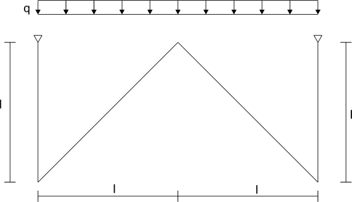
Solution
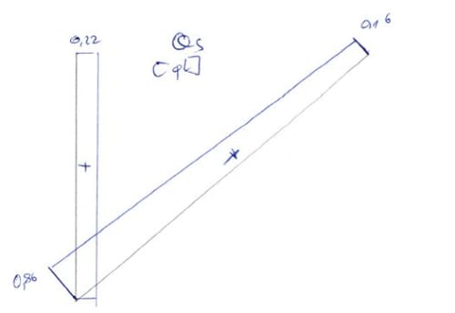
Since both the frame and the load are symmetric, I consider only the half system for symmetry.

As you can see, for this system SKN = 2
State \(\varphi_1\)
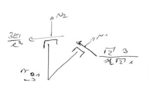
From the equilibrium of node B for moments

From the equilibrium of node C for forces

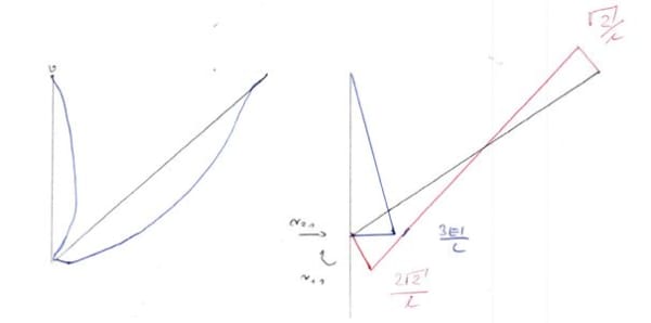
State \(\Delta_2\)


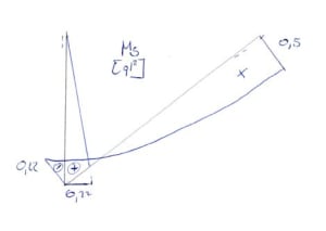
Note that from the drawing: \(sin\alpha=\frac{a}{1}\), hence \(a=\frac{1}{sin\alpha}=\sqrt2\)
From the equilibrium of node B for moments:

Result consistent with the result for state \(\varphi_1\)
From the equilibrium of nodes C and B for forces:


State P

From the equilibrium of node B for moments:
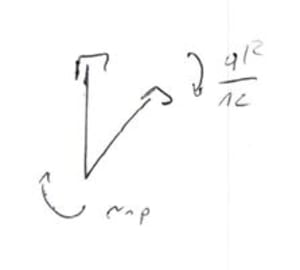 \begin{aligned}
&r_{1p}+\frac{ql^2}{12}=0\\
&r_{1p}=-\frac{ql^2}{12}\\
\end{aligned}
\begin{aligned}
&r_{1p}+\frac{ql^2}{12}=0\\
&r_{1p}=-\frac{ql^2}{12}\\
\end{aligned}
From the equilibrium of nodes B and C for forces
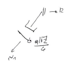

Note - due to the continuous load not perpendicular to the rod axis we have:
\begin{aligned} &N_3=N_1-ql\cdot sin\alpha\\ &\sum{F_X=0}\\ &r_{2p}+N_3\cdot cos\alpha+\frac{ql\sqrt2}{4}\cdot sin\alpha=0\\ &r_{2p}=\frac{1}{2}ql\\ \end{aligned}Substituting into the canonical equation
\begin{aligned} &r_{11}\varphi_1+r_{12}\Delta_2+r_{1p}=0\\ &r_{21}\varphi_1+r_{22}\Delta_2+r_{2p}=0\\ &5.828\frac{EI}{l}\varphi_1+7.243\frac{EI}{l^2}\Delta_2-\frac{ql^2}{12}=0\\ &7.243\frac{EI}{l^2}\varphi_1+11.486\frac{EI}{l^3}\Delta_2+\frac{1}{2}ql=0\\ \end{aligned}Hence:
\begin{aligned} &\varphi_1=0.316\frac{ql^3}{EI}\\ &\Delta_2=-0.243\frac{{ql}^4}{EI}\\ \end{aligned}From the superposition principle
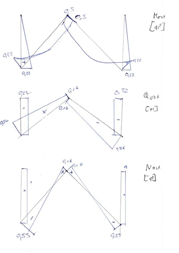
\begin{aligned} &M_{ost}=M_1\varphi_1+M_2\Delta_2+M_p\\ &M_B^A=3\frac{EI}{l^2}\cdot\Delta_2+3\frac{EI}{l^2}\cdot\varphi_1=0.22ql^2\\ &M_B^C=4.243\cdot\frac{EI}{l^2}\cdot\Delta_2+2\sqrt2\cdot\frac{EI}{l}\cdot\varphi_1-\frac{1}{12}ql^2=-0.22ql^2\\ &M_C=-4.243\cdot\frac{EI}{l^2}\cdot\Delta_2-\sqrt2\cdot\frac{EI}{l}\cdot\varphi_1-\frac{1}{12}ql^2=0.5ql^2\\ \end{aligned}Thus the graph \(M_{ost}\)
From the equilibrium of element BC
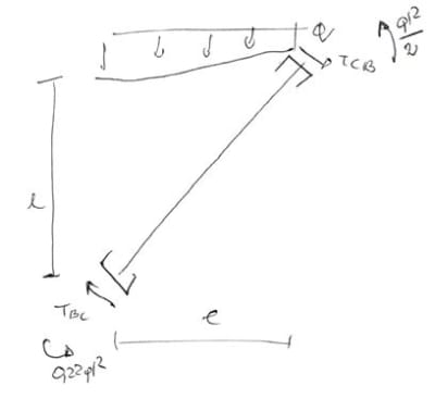 \begin{aligned}
&\sum{M_C=0}\\
&T_{BC}\cdot l\sqrt2-0.22ql^2-0.5ql^2-q\cdot l\cdot\frac{l}{2}=0\\
&T_{BC}=0.86ql\\
&\sum{M_B=0}\\
&-T_{CB}\cdot l\sqrt2-0.22ql^2-0.5ql^2+q\cdot l\cdot\frac{l}{2}=0\\
&T_{BC}=0.16ql\\
\end{aligned}
\begin{aligned}
&\sum{M_C=0}\\
&T_{BC}\cdot l\sqrt2-0.22ql^2-0.5ql^2-q\cdot l\cdot\frac{l}{2}=0\\
&T_{BC}=0.86ql\\
&\sum{M_B=0}\\
&-T_{CB}\cdot l\sqrt2-0.22ql^2-0.5ql^2+q\cdot l\cdot\frac{l}{2}=0\\
&T_{BC}=0.16ql\\
\end{aligned}
Thus the graph \(Q_{ost}\)
From the equilibrium of nodes B and C

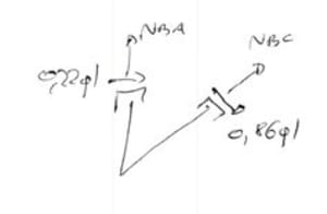
Due to the continuous load
\begin{aligned} &N_{BC}=N_{CB}-qlsin\alpha=-0.55ql\\ &\sum{F_Y=0}\\ &N_{BA}-0.86\cdot cos\alpha+N_{BC}\cdot sin\alpha=0\\ &N_{BC}=ql\\ \end{aligned}Thus the graph \(N_{ost}\)
Finally, we combine the graphs from the symmetric state, remembering that for symmetry:
- bending moments are reflected symmetrically (signs unchanged)
- shear forces are reflected antisymmetrically (signs changed to opposite)
- normal forces are reflected symmetrically (signs unchanged)