
Rozwiązanie
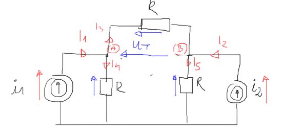 $$ I_{4} \cdot R-I_{3} \cdot R-I_{5} \cdot R=0 $$
$$ I_{4}-I_{3}-I_{5}=0 $$
$$A \quad I_{1}-I_{3}-I_{4}=0$$
$$I_{4}=I_{1}-I_{3}$$
$$B \quad I_{2}+I_{3}-I_{5}=0$$
$$I_{5}=I_{2}+I_{3}$$
$$I_{1}-I_{3}-I_{3}-\left(I_{2}+I_{3}\right)=0$$
$$-\left(3 \cdot I_{3}\right)+\left(I_{1}-I_{2}\right)=0$$
$$I_{3}=\frac{-I_{2}+I_{1}}{3}$$
\begin{aligned}
&I_{1}:=\frac{5}{\sqrt{2}} \cdot e^{1 \mathrm{j} \cdot 45 \mathrm{deg}}=2.5+2.5 \mathrm{i} \\
&I_{2}:=\frac{10}{\sqrt{2}} \cdot e^{1 \mathrm{j} \cdot 0 \mathrm{deg}}=7.071 \\
&R:=10 \\
&Z_{C}:=-1 \mathrm{j} \cdot 5=-5 \mathrm{i} \\
&I_{3}:=\frac{-I_{2}+I_{1}}{3}=-1.524+0.833 \mathrm{i} \\
&U_{T}:=I_{3} \cdot R=-15.237+8.333 \mathrm{i}
\end{aligned}
$$ I_{4} \cdot R-I_{3} \cdot R-I_{5} \cdot R=0 $$
$$ I_{4}-I_{3}-I_{5}=0 $$
$$A \quad I_{1}-I_{3}-I_{4}=0$$
$$I_{4}=I_{1}-I_{3}$$
$$B \quad I_{2}+I_{3}-I_{5}=0$$
$$I_{5}=I_{2}+I_{3}$$
$$I_{1}-I_{3}-I_{3}-\left(I_{2}+I_{3}\right)=0$$
$$-\left(3 \cdot I_{3}\right)+\left(I_{1}-I_{2}\right)=0$$
$$I_{3}=\frac{-I_{2}+I_{1}}{3}$$
\begin{aligned}
&I_{1}:=\frac{5}{\sqrt{2}} \cdot e^{1 \mathrm{j} \cdot 45 \mathrm{deg}}=2.5+2.5 \mathrm{i} \\
&I_{2}:=\frac{10}{\sqrt{2}} \cdot e^{1 \mathrm{j} \cdot 0 \mathrm{deg}}=7.071 \\
&R:=10 \\
&Z_{C}:=-1 \mathrm{j} \cdot 5=-5 \mathrm{i} \\
&I_{3}:=\frac{-I_{2}+I_{1}}{3}=-1.524+0.833 \mathrm{i} \\
&U_{T}:=I_{3} \cdot R=-15.237+8.333 \mathrm{i}
\end{aligned}
 \begin{aligned}
&I_{4}:=I_{1}-I_{3}=4.024+1.667 \mathrm{i} \\
&I_{5}:=I_{2}+I_{3}=5.547+0.833 \mathrm{i} \\
&I_{4} \cdot R-U_{T}-I_{5} \cdot R=0 \quad+ \\
&U_{T}:=I_{4} \cdot R-I_{5} \cdot R=-15.237+8.333 \mathrm{i}
\end{aligned}
\begin{aligned}
&I_{4}:=I_{1}-I_{3}=4.024+1.667 \mathrm{i} \\
&I_{5}:=I_{2}+I_{3}=5.547+0.833 \mathrm{i} \\
&I_{4} \cdot R-U_{T}-I_{5} \cdot R=0 \quad+ \\
&U_{T}:=I_{4} \cdot R-I_{5} \cdot R=-15.237+8.333 \mathrm{i}
\end{aligned}
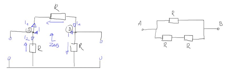 \begin{aligned}
&Z_{A B}:=\frac{R \cdot(R+R)}{R+(R+R)}=6.667 \\
&I_{2} \cdot R-I_{1} \cdot R+I_{2} \cdot R=0 \\
&I=I_{1}+I_{2} \\
&Z_{A B}=\frac{U}{I} \\
&U=I_{1} \cdot R \\
&I_{2} \cdot R+I_{2} \cdot R=I_{1} \cdot R \\
&2 I_{2}=I_{1} \\
&I=2 I_{2}+I_{2}=3 I_{2} \\
&Z_{A B}=\frac{I_{1} \cdot R}{3 I_{2}} \\
&Z_{A B}:=\frac{2}{3} R=6.667
\end{aligned}
\begin{aligned}
&Z_{A B}:=\frac{R \cdot(R+R)}{R+(R+R)}=6.667 \\
&I_{2} \cdot R-I_{1} \cdot R+I_{2} \cdot R=0 \\
&I=I_{1}+I_{2} \\
&Z_{A B}=\frac{U}{I} \\
&U=I_{1} \cdot R \\
&I_{2} \cdot R+I_{2} \cdot R=I_{1} \cdot R \\
&2 I_{2}=I_{1} \\
&I=2 I_{2}+I_{2}=3 I_{2} \\
&Z_{A B}=\frac{I_{1} \cdot R}{3 I_{2}} \\
&Z_{A B}:=\frac{2}{3} R=6.667
\end{aligned}
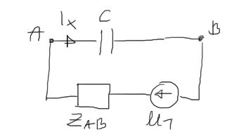 \begin{aligned}
&I_{x}:=\frac{U_{T}}{Z_{A B}+Z_{C}}=-2.063-0.297 \mathrm{i} \\
&I_{x}=2.084 \angle-2.999
\end{aligned}
\begin{aligned}
&I_{x}:=\frac{U_{T}}{Z_{A B}+Z_{C}}=-2.063-0.297 \mathrm{i} \\
&I_{x}=2.084 \angle-2.999
\end{aligned}
Jeżeli masz jakieś pytania, uwagi lub wydaje Ci się, że znalazłeś błąd w tym rozwiązaniu, napisz proszę do nas wiadomość na kontakt@edupanda.pl lub skontaktuj się z nami przez nasz profil na FB: